Executes one prediction and correction step of the MEKF.
This function propagates the state forward using gyroscope readings (prediction step) and then corrects the estimate using magnetometer data (correction step).
91{
92 static const double Q[36] = {4.3956900000000333E-11,
93 0.0,
94 0.0,
95 -5.0000000000000008E-23,
96 -0.0,
97 -0.0,
98 0.0,
99 4.3956900000000333E-11,
100 0.0,
101 -0.0,
102 -5.0000000000000008E-23,
103 -0.0,
104 0.0,
105 0.0,
106 4.3956900000000333E-11,
107 -0.0,
108 -0.0,
109 -5.0000000000000008E-23,
110 -5.0000000000000008E-23,
111 -0.0,
112 -0.0,
113 1.0000000000000001E-20,
114 0.0,
115 0.0,
116 -0.0,
117 -5.0000000000000008E-23,
118 -0.0,
119 0.0,
120 1.0000000000000001E-20,
121 0.0,
122 -0.0,
123 -0.0,
124 -5.0000000000000008E-23,
125 0.0,
126 0.0,
127 1.0000000000000001E-20};
128 static const double dv[11] = {23950.03, 23938.16, 23926.3, 23914.44,
129 23902.6, 23890.76, 23878.93, 23867.11,
130 23855.29, 23843.49, 23831.69};
131 static const double dv1[11] = {2585.64, 2583.71, 2581.78, 2579.85,
132 2577.92, 2576.0, 2574.08, 2572.15,
133 2570.24, 2568.32, 2566.4};
134 static const double dv2[11] = {39593.08, 39573.32, 39553.57, 39533.84,
135 39514.11, 39494.41, 39474.71, 39455.03,
136 39435.36, 39415.7, 39396.06};
137 static const double b_y[9] = {0.01, 0.0, 0.0, 0.0, 0.01, 0.0, 0.0, 0.0, 0.01};
139 static const signed char iv[18] = {0, 0, 0, 0, 0, 0, 0, 0, 0,
140 1, 0, 0, 0, 1, 0, 0, 0, 1};
141 static const signed char b[9] = {1, 0, 0, 0, 1, 0, 0, 0, 1};
142 double Phi[36];
143 double b_Phi[36];
144 double H[18];
145 double K[18];
146 double b_H[18];
147 double cos_term[16];
148 double A[9];
149 double dv3[9];
150 double skew_omega_sq[9];
151 double delta_x[6];
152 double delta_q[4];
153 double axis[3];
154 double b_W[3] = {0};
155 double A_tmp;
156 double a;
157 double angle;
158 double b_a;
159 double d;
160 double omega_norm;
161 double sin_term;
162 double x;
163 double y;
164 int H_tmp;
165 int b_i;
166 int cos_term_tmp;
167 int i;
168
169
170
171
172
173
174
175
176
177
178
179
180
181
182
183
184
185
186
187
188
189 y = floor(height_AGL / 1000.0);
190 omega_norm = ceil(height_AGL / 1000.0);
191
192
193
194
195
196
197
198
199
200
201 y = 2.0 * (
q[2] *
q[2]);
202 omega_norm = 2.0 * (
q[1] *
q[1]);
203 A[0] = (1.0 - omega_norm) - y;
205 sin_term =
q[2] *
q[3];
206 A[3] = 2.0 * (x - sin_term);
209 A[6] = 2.0 * (A_tmp + angle);
210 A[1] = 2.0 * (x + sin_term);
211 x = 1.0 - 2.0 * (
q[0] *
q[0]);
212 A[4] = x - y;
214 sin_term =
q[0] *
q[3];
215 A[7] = 2.0 * (y - sin_term);
216 A[2] = 2.0 * (A_tmp - angle);
217 A[5] = 2.0 * (y + sin_term);
218 A[8] = x - omega_norm;
219
220
221
222 H[0] = 0.0;
223 H[4] = 0.0;
224 H[8] = 0.0;
225 d = b_W[0];
226 A_tmp = b_W[1];
227 y = b_W[2];
228 for (i = 0; i < 3; i++) {
229 H_tmp = 3 * (i + 3);
230 H[H_tmp] = 0.0;
231 H[H_tmp + 1] = 0.0;
232 H[H_tmp + 2] = 0.0;
233 axis[i] = (A[i] * d + A[i + 3] * A_tmp) + A[i + 6] * y;
234 }
235 H[3] = -axis[2];
236 H[6] = axis[1];
237 H[1] = axis[2];
238 H[7] = -axis[0];
239 H[2] = -axis[1];
240 H[5] = axis[0];
241
242 for (i = 0; i < 3; i++) {
243 for (cos_term_tmp = 0; cos_term_tmp < 6; cos_term_tmp++) {
244 d = 0.0;
245 for (H_tmp = 0; H_tmp < 6; H_tmp++) {
246 d += H[i + 3 * H_tmp] * P[H_tmp + 6 * cos_term_tmp];
247 }
248 b_H[i + 3 * cos_term_tmp] = d;
249 }
250 for (cos_term_tmp = 0; cos_term_tmp < 3; cos_term_tmp++) {
251 d = 0.0;
252 for (H_tmp = 0; H_tmp < 6; H_tmp++) {
253 d += b_H[i + 3 * H_tmp] * H[cos_term_tmp + 3 * H_tmp];
254 }
255 H_tmp = i + 3 * cos_term_tmp;
256 skew_omega_sq[H_tmp] = d + (double)
R[H_tmp];
257 }
258 }
259 mpower(skew_omega_sq, dv3);
260 for (i = 0; i < 6; i++) {
261 for (cos_term_tmp = 0; cos_term_tmp < 3; cos_term_tmp++) {
262 d = 0.0;
263 for (H_tmp = 0; H_tmp < 6; H_tmp++) {
264 d += P[i + 6 * H_tmp] * H[cos_term_tmp + 3 * H_tmp];
265 }
266 b_H[i + 6 * cos_term_tmp] = d;
267 }
268 d = b_H[i];
269 A_tmp = b_H[i + 6];
270 y = b_H[i + 12];
271 for (cos_term_tmp = 0; cos_term_tmp < 3; cos_term_tmp++) {
272 K[i + 6 * cos_term_tmp] =
273 (d * dv3[3 * cos_term_tmp] + A_tmp * dv3[3 * cos_term_tmp + 1]) +
274 y * dv3[3 * cos_term_tmp + 2];
275 }
276 }
277
280
281 omega_norm = 0;
282 x = 0;
283 y = 0;
284
285
286
287
288
289
290
291
292
293
294
295
296
298 for (i = 0; i < 6; i++) {
299 d = K[i];
300 A_tmp = K[i + 6];
301 y = K[i + 12];
302 delta_x[i] = (d * b_W[0] + A_tmp * b_W[1]) + y * b_W[2];
303 for (cos_term_tmp = 0; cos_term_tmp < 6; cos_term_tmp++) {
304 H_tmp = i + 6 * cos_term_tmp;
305 b_Phi[H_tmp] =
306 Phi[H_tmp] -
307 ((d * H[3 * cos_term_tmp] + A_tmp * H[3 * cos_term_tmp + 1]) +
308 y * H[3 * cos_term_tmp + 2]);
309 }
310 for (cos_term_tmp = 0; cos_term_tmp < 6; cos_term_tmp++) {
311 d = 0.0;
312 for (H_tmp = 0; H_tmp < 6; H_tmp++) {
313 d += b_Phi[i + 6 * H_tmp] * P[H_tmp + 6 * cos_term_tmp];
314 }
315 Phi[i + 6 * cos_term_tmp] = d;
316 }
317 }
318 delta_q[0] = 0.5 * delta_x[0];
319 delta_q[1] = 0.5 * delta_x[1];
320 delta_q[2] = 0.5 * delta_x[2];
322 ((delta_q[0] *
q[3] +
q[0]) +
q[1] * delta_q[2]) - delta_q[1] *
q[2];
324 ((delta_q[1] *
q[3] -
q[0] * delta_q[2]) +
q[1]) + delta_q[0] *
q[2];
326 ((delta_q[2] *
q[3] +
q[0] * delta_q[1]) - delta_q[0] *
q[1]) +
q[2];
328 ((
q[3] -
q[0] * delta_q[0]) -
q[1] * delta_q[1]) -
q[2] * delta_q[2];
337 memcpy(&P[0], &Phi[0], 36U * sizeof(double));
338
339
343
345
346 angle = omega_norm * 0.01;
347
348 x = cos(angle);
349 sin_term = sin(angle);
350
351
352 A[0] = 0.0;
353 A[3] = -b_W[2];
354 A[6] = b_W[1];
355 A[1] = b_W[2];
356 A[4] = 0.0;
357 A[7] = -b_W[0];
358 A[2] = -b_W[1];
359 A[5] = b_W[0];
360 A[8] = 0.0;
361
362 for (b_i = 0; b_i < 3; b_i++) {
363 axis[b_i] = b_W[b_i] / omega_norm;
364 for (i = 0; i < 3; i++) {
365 skew_omega_sq[b_i + 3 * i] =
366 (A[b_i] * A[3 * i] + A[b_i + 3] * A[3 * i + 1]) +
367 A[b_i + 6] * A[3 * i + 2];
368 }
369 }
370
371 a = sin_term / omega_norm;
372 y = omega_norm * omega_norm;
373 b_a = x / y;
374 x = (1.0 - x) / y;
375 y = (angle - sin_term) /
rt_powd_snf(omega_norm, 3.0);
376
378 for (i = 0; i < 3; i++) {
379 d = A[3 * i];
380 A_tmp = skew_omega_sq[3 * i];
381 Phi[6 * i] = (dv3[3 * i] - a * d) + b_a * A_tmp;
382 H_tmp = 6 * (i + 3);
383 Phi[H_tmp] = (x * d - y * A_tmp) - b_y[3 * i];
384 cos_term_tmp = 3 * i + 1;
385 d = A[cos_term_tmp];
386 A_tmp = skew_omega_sq[cos_term_tmp];
387 Phi[6 * i + 1] = (dv3[cos_term_tmp] - a * d) + b_a * A_tmp;
388 Phi[H_tmp + 1] = (x * d - y * A_tmp) - b_y[cos_term_tmp];
389 cos_term_tmp = 3 * i + 2;
390 d = A[cos_term_tmp];
391 A_tmp = skew_omega_sq[cos_term_tmp];
392 Phi[6 * i + 2] = (dv3[cos_term_tmp] - a * d) + b_a * A_tmp;
393 Phi[H_tmp + 2] = (x * d - y * A_tmp) - b_y[cos_term_tmp];
394 }
395 for (i = 0; i < 6; i++) {
396 Phi[6 * i + 3] = iv[3 * i];
397 Phi[6 * i + 4] = iv[3 * i + 1];
398 Phi[6 * i + 5] = iv[3 * i + 2];
399 }
400
401
402
403 for (i = 0; i < 6; i++) {
404 for (cos_term_tmp = 0; cos_term_tmp < 6; cos_term_tmp++) {
405 d = 0.0;
406 for (H_tmp = 0; H_tmp < 6; H_tmp++) {
407 d += Phi[i + 6 * H_tmp] * P[H_tmp + 6 * cos_term_tmp];
408 }
409 b_Phi[i + 6 * cos_term_tmp] = d;
410 }
411 for (cos_term_tmp = 0; cos_term_tmp < 6; cos_term_tmp++) {
412 d = 0.0;
413 for (H_tmp = 0; H_tmp < 6; H_tmp++) {
414 d += b_Phi[i + 6 * H_tmp] * Phi[cos_term_tmp + 6 * H_tmp];
415 }
416 H_tmp = i + 6 * cos_term_tmp;
417 P_new[H_tmp] = d +
Q[H_tmp];
418 }
419 }
420
421
422
423 x = cos(0.5 * angle);
424 sin_term = sin(0.5 * angle);
425
426
427 skew_omega_sq[0] = sin_term * 0.0;
428 skew_omega_sq[3] = sin_term * -axis[2];
429 skew_omega_sq[6] = sin_term * axis[1];
430 skew_omega_sq[1] = sin_term * axis[2];
431 skew_omega_sq[4] = sin_term * 0.0;
432 skew_omega_sq[7] = sin_term * -axis[0];
433 skew_omega_sq[2] = sin_term * -axis[1];
434 skew_omega_sq[5] = sin_term * axis[0];
435 skew_omega_sq[8] = sin_term * 0.0;
436 for (b_i = 0; b_i < 3; b_i++) {
437 d = sin_term * axis[b_i];
438 H_tmp = b_i << 2;
439 cos_term[H_tmp] = x * (double)b[3 * b_i] - skew_omega_sq[3 * b_i];
440 cos_term_tmp = 3 * b_i + 1;
441 cos_term[H_tmp + 1] =
442 x * (double)b[cos_term_tmp] - skew_omega_sq[cos_term_tmp];
443 cos_term_tmp = 3 * b_i + 2;
444 cos_term[H_tmp + 2] =
445 x * (double)b[cos_term_tmp] - skew_omega_sq[cos_term_tmp];
446 cos_term[b_i + 12] = d;
447 cos_term[H_tmp + 3] = -d;
448 }
449 cos_term[15] = x;
453 omega_norm =
q_new[3];
454 for (i = 0; i < 4; i++) {
455 delta_q[i] =
456 ((cos_term[i] * d + cos_term[i + 4] * A_tmp) + cos_term[i + 8] * y) +
457 cos_term[i + 12] * omega_norm;
458 }
459
461 q_new[0] = delta_q[0] / d;
462 q_new[1] = delta_q[1] / d;
463 q_new[2] = delta_q[2] / d;
464 q_new[3] = delta_q[3] / d;
465}
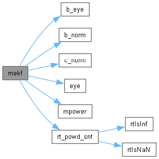
void b_eye(double b_I[36])
Creates a 6x6 identity matrix.
void eye(double b_I[9])
Creates a 3x3 identity matrix.
static double rt_powd_snf(double u0, double u1)
void mpower(const double a[9], double c[9])
Calculates the inverse of a 3x3 matrix.
double b_norm(const double x[3])
Calculates the Euclidean norm (magnitude) of a 3-element vector.
double c_norm(const double x[4])
Calculates the Euclidean norm (magnitude) of a 4-element vector.